Lab 4: Simulation of a RISC-V based SoC using GVSoC
Welcome to lab 4, the last lab of this course. In this lab, we will use the GVSoC simulator to simulate a RISC-V based SoC. You will be implementing the same Scaled Indexed (SI) Load instruction as you did in lab 2 to get you started. And then, you will be extending the functionality of the RISC-V core to support multi-core processing.
The VM password is
celab4.
Table of Contents
- Learning goals of the lab
- Setting up the virtual machine and getting the lab template files
- Part 1: Implementing the Load Word Indexed (LWI) instruction
- Part 2: Extending the RISC-V core to support multi-core processing
- Verification & Profiling
- BONUS: Run a character histogram algorithm with the multi-core processor
Learning goals of the lab
Simulators are a helpful tool to understand the behavior of a processor and its components. They allow for a faster design space exploration (DSE) than other tools (like Vivado) and can be used to test new features and functionalities with a subset of relevant system parameters, making them very versatile.
This lab will introduce you to the GVSoC simulator and teach you how custom changes are made, such as adding an instruction and changing the execution to multi-core.
 Main parts that compose GVSoC: JSON files describe the architecture, Python generators instantiate the components and C++ models describe all the IPs (b) How GVSoC components interact with each other. Every component receives a request containing the information to forward it to another component or to handle it by itself.")
Setting up the virtual machine and getting the lab template files
This section will guide you on how to install the VirtualBox virtual machine for the labs on your own laptop. The virtual machine is pre-configured with all the necessary tools and libraries for the labs: the compiled riscv-gnu-toolchain, GVSoC and their dependencies.
Using the desktop computers: If you are using the lab desktop computers, the VM image is already loaded in the shared folder. Jump to step 3.
Step 1: Download VirtualBox in the following link Virtual box 7.0.16. This is the same VirtualBox version used in the lab desktop computers.
Step 2: Download the VM image from the following link: VM image
Step 3: To import the VM image. Open VirtualBox and click on Tools > Import. In the import wizard, click on the folder icon to select the ce-lab4.ova image that you downloaded and click Next.
On Lab Desktops, the
ce-lab4.ovafile is located atC:\Programs\CESE4130

You can now change the number of CPU's and RAM allocated for the machine (For the desktop computers, decrease the number of cores to 4 and keep the RAM the same), and click Finish. Once the machine is done importing, you will see it appear on the left-hand side, from where you can Start it.
The root password for the VM is celab4.
Step 4: Once you start the machine. Open a terminal and go to the developer directory, get the template files for this lab and unzip them using these commands:
cd ~/trial2/gvsoc/docs/developer/
curl https://cese.ewi.tudelft.nl/computer-engineering/docs/CESE4130_Lab4.zip --output CESE4130_Lab4.zip
unzip CESE4130_Lab4.zip -d cese4130-lab4/
Part 1: Implementing the Load Word Indexed (LWI) instruction
In this Part, you will be adding the same Scaled Indexed Load instruction you implemented in Lab 2, formally known as Load Word Indexed (LWI). To add this custom instruction to the RISC-V core, you will have to modify the python generator file for RISC-V and one of the ISA header codes of the processor. To verify the implementation, you will run the image blur algorithm with the original ISA and the modified ISA.
If you did not get the lab files yet, go back to the previous section: setting up the virtual machine and getting the lab template files.
Running the Image blur algorithm with the original ISA
Before you add the instruction, run the image blur algorithm with the original ISA to see the current number of cycles it takes to execute.
-
Go into the baseline directory:
cd ~/trial2/gvsoc/docs/developer/cese4130-lab4/img-blur-baseline -
Compile the GVSoC core, the image blur algorithm and count the amount of cycles it takes to run the image blur algorithm:
make gvsoc all count-cycles -
Note down the number of cycles it took to run the image blur algorithm, shown on your terminal.
Adding the instruction
Python generator decoder
Now, let's add the instruction format to be decoded by the processor in the python file.
-
Navigate to the specific RISC-V generator file
~/trial2/gvsoc/core/models/cpu/iss/isa_gen/isa_riscv_gen.py -
Add your decoding to the
initfunction of theRv32iclass. We will not set thefast-handler.
The instruction is encoded as follows:
| 31 ... 25 | 24 ... 20 | 19 ... 15 | 14 ... 12 | 11 ... 7 | 6 ... 0 |
|---|---|---|---|---|---|
| funct7 | rs2 | rs1 | funct3 | rd | opcode |
| 0000000 | rs2 | rs1 | 010 | rd | 0101011 |
- func7 (7-bits): A constant field containing
'0000000'. - rs2 (5-bits): Specifies the index register.
- rs1 (5-bits): Specifies the base register.
- func3 (3-bits): A constant field containing
'010'. - rd (5-bits): Specifies the destination register.
- opcode (7-bits): The opcode for this custom instruction containing
'0101011'.
Leading to the assembly format: 'lwi <rd>,<rs2>,<rs1>'. Slightly different from lab 2 because of GVSoC conversions.
Where <rd>, <rs1>, and <rs2> placeholders denote the fields which specify the destination, base, and index registers, respectively.
Hint: You can use the
lwandaddinstruction as a reference to implement thelwiinstruction. Because thelwiinstruction also needs to behave as an addition, it is not L type.
ISA header code
- Navigate to
~/trial2/gvsoc/core/models/cpu/iss/include/isa/rv32i.hpphere you will find how instructions of this subset are defined. - Include a function with the same format of the others called
lwi_execwith the execution of the LWI instruction.
Hint: You can use the
lwandaddinstruction as a reference to implement thelwiinstruction.
Check if you added your instruction correctly
-
Navigate to the 'check-img-blur-modified' directory
cd ~/trial2/gvsoc/docs/developer/cese4130-lab4/check-img-blur-modified
There you will find:
- The original image used to create the assembly file, and
- The assembly file that tests the lwi instruction
-
Run the following command to check if you are blurring the image correctly
make gvsoc all run imageYou can then check the output image and the
data.txtoutput file that will confirm if your image was blurred correctly.
Running the Image blur algorithm with the modified ISA
Now that you implemented and tested your instruction, lets compare by running the same image blur algorithm.
-
Navigate to the 'img-blur-modified' directory:
cd ~/trial2/gvsoc/docs/developer/cese4130-lab4/img-blur-modified` -
Run the following command to compile the GVSoC core, the image blur algorithm and count the amount of cycles it takes to run the image blur algorithm:
make gvsoc all count-cycles -
Note down the number of cycles it took to run the image blur algorithm
Question
What is the difference in the number of cycles it took to run the image blur algorithm with the original ISA and the modified ISA?
Part 2: Extending the RISC-V core to support multi-core processing
In this Part you will be experimenting with simulating a multi-core system. You will modify your SoC by adding additional cores, and then modify the C program to make it parallel in your RISC-V core.
As a parallelizable workload, you will be counting the number of 3s in an predefined array.
Running the Baseline
-
Navigate to the Part 2 directory on your VM:
cd ~/trial2/gvsoc/docs/developer/cese4130-lab4/Part-2 -
Choose an array to run the program with: There are 3 predefined arrays provided in
main.cfile. You can set theARRAYdefinition to select between the arrays. In the following section these arrays are referred to as Array-1, Array-2, and Array-3.// ************************* Test Arrays ************************* #ifndef ARRAY #define ARRAY 1 #endif #if (ARRAY == 1) // ARRAY-1; 1000 elements; 56 occurances of 3 const uint32_t arr[] = { 15, 10, 1, 19, 16, 9, 9, 18, 4, 15, ... #elif(ARRAY == 2) // ARRAY-2; 1000 elements; 0 occurrences of 3 const uint32_t arr[] = { 15, 10, 1, 19, 16, 9, 9, 18, 4, 15, ... #else // ARRAY-3; 36 elements; 12 occurrences of 3 const uint32_t arr[] = {1,2,3,1,2,3,1,2,3,1,2,3,1,2,3,1,2,3,1 ... #endif // **************************************************************** -
To run the baseline you need to make the GVSoC simulator, then compile the code and run it. This can be done using the command below:
make gvsoc all run -
You should be able to see the following expected output on your terminal:
The total 3s are:56
Adding the cores
Since we are simulating a multi-core system, you need to define the cores in your system. To do this you will be modifying my_system.py
Understand how a core is defined in GVSoC
A core is defined as an module in GVSoC. You can use a pre-defined core or generate a custom core using the generators. For this exercise we will be using the generic RISC-V core provided with GVSoC. A core is normally defined inside a SoC (System-on-Chip), and involves 3 main steps:
-
Definition of the core: Here you instantiate a variable with the core class. You set the core name (
hostin this case), the instruction set architecture (isa) to be executed by the core and thecore_idhost = cpu.iss.riscv.Riscv(self, 'host', isa='rv64imafdc', core_id = 0) -
Connecting to Memory: The core is connected to the main memory inside the SoC. In our example the instruction and data memory are stored in a single memory component.
host.o_FETCH ( ico.i_INPUT ()) host.o_DATA ( ico.i_INPUT ()) host.o_DATA_DEBUG( ico.i_INPUT ()) -
Loading the program on the core: In GVSoC the compiled
.elffile is loaded into the memory using theloader. Thus, each core needs to be connected to a loader.loader.o_START ( host.i_FETCHEN ()) loader.o_ENTRY ( host.i_ENTRY ())
Adding multiple cores
To add new cores, you need to follow the three steps mentioned in the previous section. You can duplicate the core instantiation, connection to memory and loader to generate a new core in your SoC.
Note: Each core should have a different name and core_id
For this assignment you need to define a total of 16 cores.
Connecting to the Global Memory
For our multi-core system, you are provided with a custom component called global memory. It is used to simulate a memory that is shared with all the cores. You should not change the already declared memory.
To connect the new component to your Soc, you need to follow the steps:
-
Create an object of the component: Refer to
global_mem.pyto see how the class is declared and the arguments required for the constructor -
Map the component to the interconnect: For the cores to access the global memory, you need to map it to a know address range. You can refer to the main memory to see how a component is mapped to the interconnect.
ico.o_MAP(mem.i_INPUT(), 'mem', base=0x00000000, size=0x00100000, rm_base=True)Map the component with the following parameters:
- Base address: 0x20000000
- Size: 0x00001000
Once completed, run
make gvsocto compile your custom SoC and check for errors
Parallelize the program
The program provided in main.c is implemented to run on a single core. Unlike the previous Lab (CUDA), you will be programming directly on the simulated RISC-V core. Which means there are no pre-defined functions like __syncthreads(), you will have to implement them by yourself.
The program is elaborated in the workflow below:
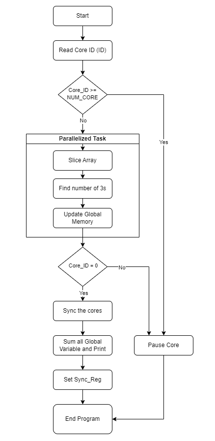
Some key steps required for the multi-core system are provided in the template program. You need to uncomment them after you have finished the modifications in my_system.py.
You need to divide the array between the cores to optimize the core useage. And print the final result correctly.
To run your program you can set the number of cores using:
// Define the number of cores you want to simulate with
#ifndef NUM_CORES
    #define NUM_CORES 1
#endif
Once completed, you can run make all to compile the solution, and make run to execute the solution.
Hint: If you don't see any output in the terminal, check if all the cores are being paused correctly, until Core-0 finishes execution
Verification & Profiling
To verify your program and the core implementation run the following command:
make gvsoc verify
Once the verification is completed successfully you con continue with profiling and answering the questions.
Note: You will need to show the verification output to the TAs during sign-off
Profiling
Set ARRAY 1 and run make plot. This will make a plot between execution-cycles vs. number of cores. Using this plot, answer the following questions:
- Why is the graph non-linear?
- Apply Amdahl's Law on the program using the values in the graph, and calculate the percentage of the code that is parallelizable. You may want to use the following lecture slides: Slide 11
Amdahl's law : $$ Speed up_{max} = {1 \over {(1-p)} + ({p \over s})}$$
Where
- Speed up is the maximum speedup of the system
- p is part of the system that is improved
- s is the speedup of p
- What will be the future trend of the plot if the cores are increased beyond 16?
Set ARRAY 2 and run make diff. The main difference in Array-1 and Array-2 is that there are no 3s in Array-2. Thus you need to analyze how the absence of 3s affects the execution cycles in a multi-core system. To facilitate this analysis, make diff plots the difference in execution cycles for Array-1 and Array-2. Answer the following questions based on your observations of the graph.
- Based on the program in
main.cwhat is the difference in execution for Array-1 and Array-2? - Why is the difference in number of cycles between Array-1 and Array-2 decreasing? Will the difference reach zero if the cores are increased?
- How will the difference change if the number of occurrences are more in Array-1?
Set ARRAY 3 and run make plot. This will make a plot between execution-cycles vs. number of cores. Using this plot, answer the following questions:
- Why is the trend for this plot different from the previous plots?
- For this array what will be the ideal number of cores to execute the program?
BONUS: Run a character histogram algorithm with the multi-core processor
To give everyone a fair chance to check the first two parts, the bonus will only be accepted until 12:30 and after you already signed off Parts 1 and 2.
As the bonus task for this last lab, you will be extending the implementation that you used for Part 2. More specifically, to compute a character histogram. Like the one you did in Lab 3 - Part 3.
First, you need to copy the changes you made to the Part2/my_system.py file to the bonus/my_system.py file. Then, you need to implement the character histogram algorithm in the main.c file, just like you did in Part 2, but taking NUM_BINS into account.
A small and big test arrays are given to you in the main.c file. You can choose to test the program with either of them. The sign off will happen using the big test array.
Once you have implemented the character histogram algorithm, you can run the following command to compile and run the program:
make gvsoc all run
You should see the output of the character histogram in the terminal. To plot and make sure your multi-core implementation is correct, you can run the following command:
make plot
Show your terminal output and the plot to the TAs for the sign-off.